Foreword
I started getting emails after I first wrote this article every year at around the start of the NBA season from people wanting to buy this model. In 2022, I built another website, https://www.FantaZscores.com, to sell it. If you wish to buy the model you can do so there.
This case is split into two parts. The first section, Analysis, discusses the high level implications of my findings. The second section, Technical Process, goes through the step by step code that I used to generate these insights.
I've tried to keep this case understandable even if you don't know anything about fantasy basketball. So don't worry if you're not a big basketball fan!
Analysis
Welcome to Moneyball for the NBA, today I'll be your Jonah Hill. We're going to analyze how we can build a fantasy basketball team that's better and cheaper than can be drafted without analytics.
But wait... Let me explain a few basics first. The premise of Fantasy Basketball is simple; each person participating in the league will select real NBA players to compose their 'fantasy team'. Fantasy teams will then compete against each other - winning and losing based on the real life performances of the NBA players on those fantasy teams. This is the story of how I broke our 2017-18 league using data analytics.
The future of every fantasy basketball team is made or broken on draft day. If you draft your team well you will be set up for a season of success, and if you draft poorly, it is nearly impossible to recover.
Typically, in fantasy sports, league members will take turns drafting players sequentially until a given number of required players is reached. But in 2017, my league decided to move away from this set up, opting instead to use a live auction for player selection. This set the foundation for the strategy that I'll lay out in this analysis.
Here's how the live auction works:
- Each league member is alloted \$200 (not real money) to draft players to create their team
- Each team consists of 13 NBA players
- On draft day, NBA players are nominated one by one and league members are able to bid from their \$200 pool of money to purchase that player for their team. Whoever is willing to bid the most for a player will purchase that player for their team
- The auction is live, meaning that if I bid \$50 on a player, everyone else will see my bid and will have 10 seconds to bid a higher amount before my bid purchases that player.
Now that we understand how the draft works, we need to decide who we are targetting and how much we should be willing to pay for them.
Well luckily, Yahoo, the largest fantasy sports
platform, provides projected player values that
they believe players should be bought for. They
also provide the average value that players are
actually being drafted for, as seen below.
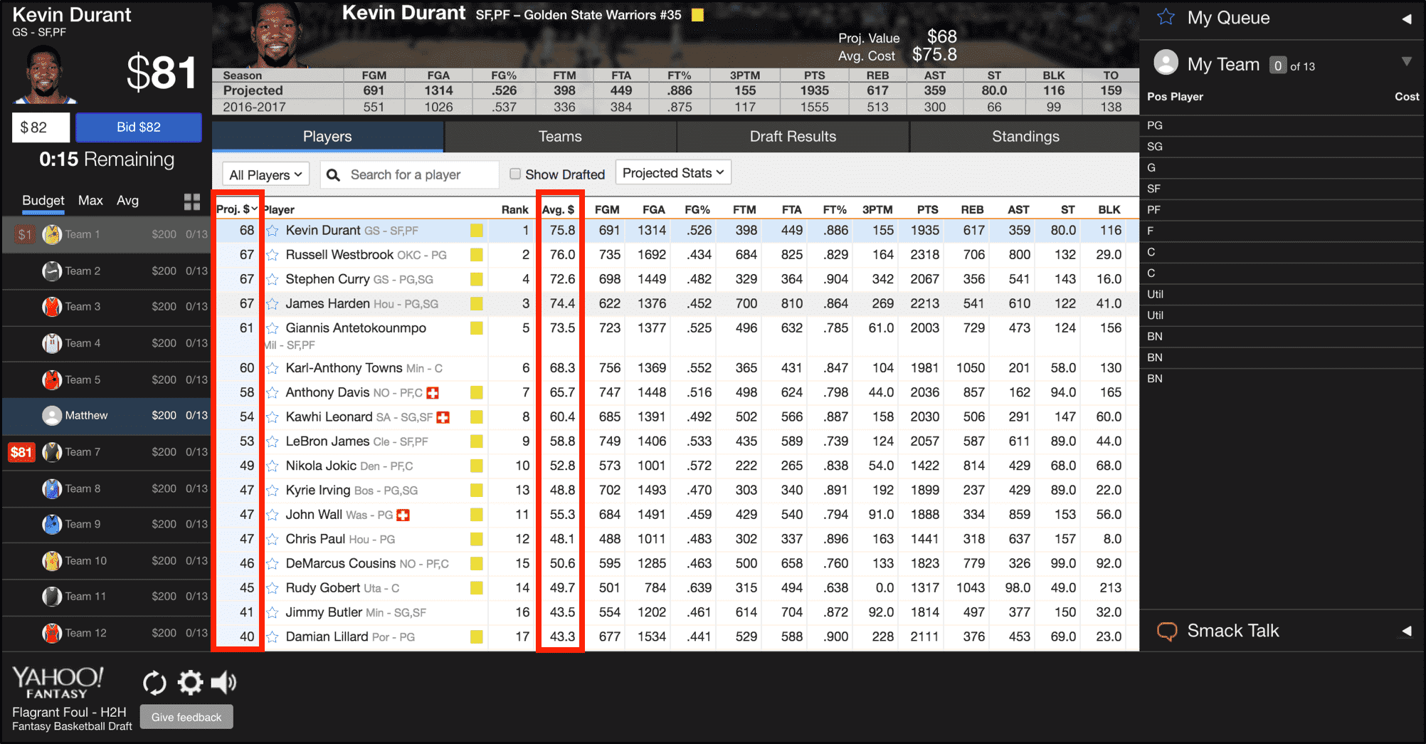
Yahoo's projected values are treated as the gold
standard among fantasy basketball players. These
values are used as a baseline for decision
making during the draft. For instance, if we
think a player is underrated, we may be willing
to bid \$5 - \$10 higher than Yahoo's projected
value.
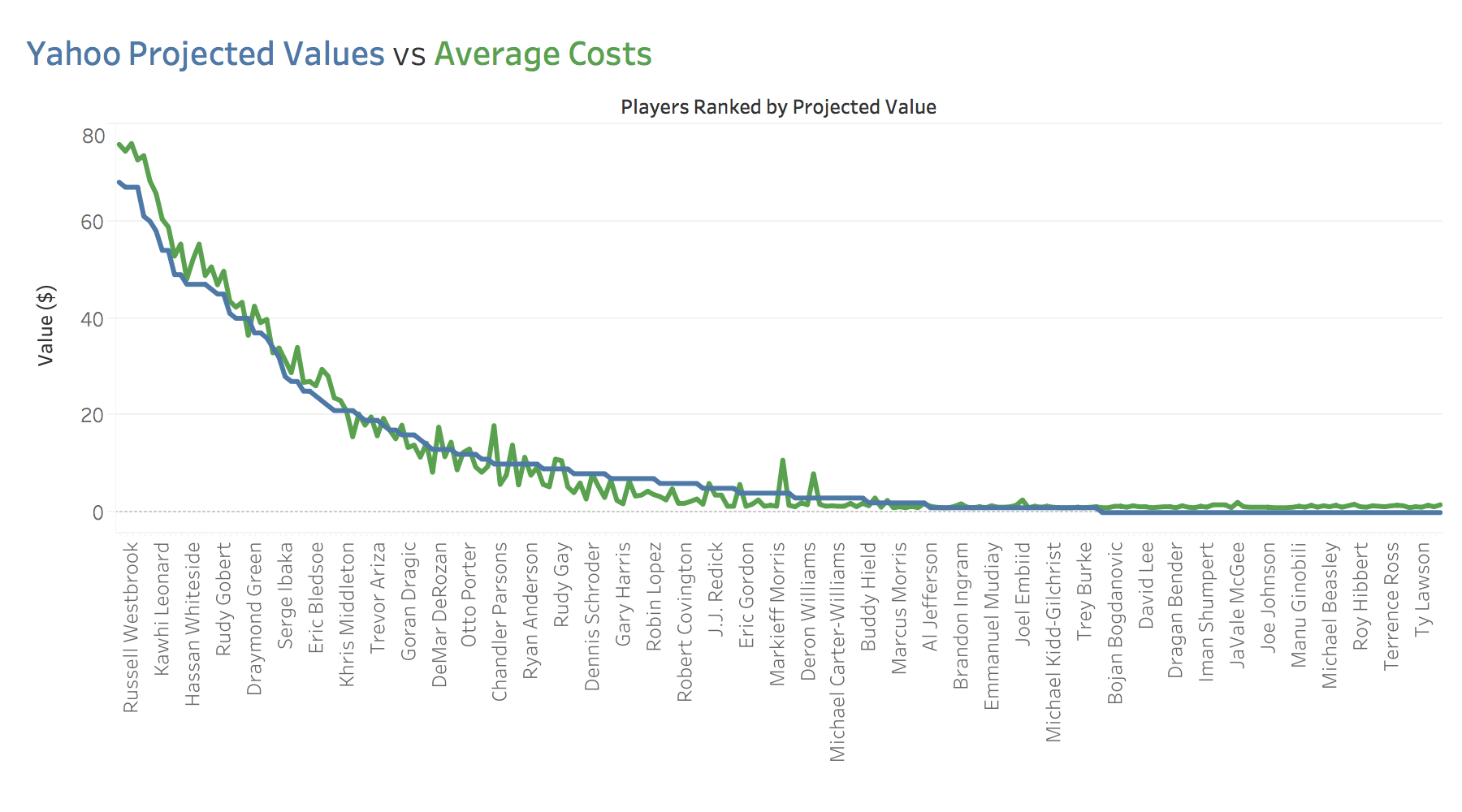
But don't take my word for that - take a look at
the graph below showing the difference between
Yahoo's projected values and actual draft values
for each player. The average draft values follow
Yahoo's projected values extremely closely.
This begs the question though - if everyone is
blindly basing their decisions on Yahoo's
projected values -
how do we know if those values are
accurate? Well, we don't. We have absolutely no idea
where those numbers are coming from or how they
are generated.
Ok, so since we don't know where the Yahoo numbers come from, I thought it might be helpful to develop a metric for scoring players and assigning them dollar values. This would allow us to compare our values against Yahoo's projections to determine if the Yahoo projections are accurate. But if I'm going to come up with my own method for valuing NBA players, I need to make sure that it is mathematically accurate.
Luckily, we can use z-scores to perform a mathematical evaluation of NBA players from their previous season's statistics and then we can use those z-scores to derive a dollar value that we can compare against Yahoo's projections. If you're interested in the details of these calculations, you can see them in the Technical Process section below.
Here's a quick and dirty overview of why z-scores work - skip this if you don't like math. Z-scores take the NBA average from the previous season across each relevant stat (points, rebounds, assists, etc) and then calculate how many standard deviations from the mean each player falls in each category. Then, we average their z-score across all categories to come up with a weighted score. We can then add up the weighted scores for the top 150 or so players depending on how many players will be in the league, and then apply their fraction of the total weighted values to the total number of dollars available for spending in the league. Boom - mathematically accurate player values calculated.
Math, calculations, and z-scores sound pretty
complicated though. And they never mention
anything like that in Moneyball so why do we
even need them? Well, here's what you need to
know - the red line in the graph below is a
mathematically accurate assessment of what
players are worth. At times, that red line is
far away from the green line which is what
players actually cost. If the red line is above
the green line, then players are mathematically
worth more than what they are being sold for. We
can buy those players at a discount from what
they are actually worth.
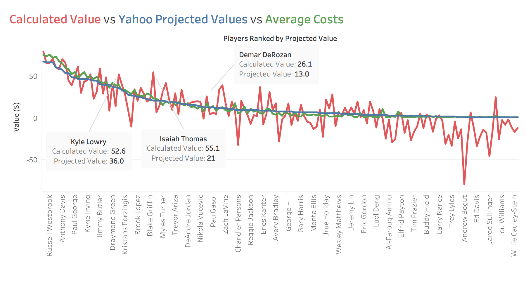
I know, I know, you are probably thinking that
previous season stats aren't forward looking and
therefore don't account for factors such as
player injuries or trades. That is definitely
true, shown above, Isaiah Thomas is calculated
to be worth \$55.1 from his previous season
stats but after injuring his hip between seasons
and being traded to another team, his projected
value decreased by over 50% to \$21.0. That
seems justified and goes to show that we still
need to examine individual player situations
before assuming this data is completely
accurate.
But in the majority of cases there is seemingly no reason for Yahoo's projected values to be so different from the previous year. Take Toronto's two star players during the 2016-17 season, Kyle Lowry and Demar DeRozan. Both will be playing in nearly the same situation in 2017-18 and injuries are not a major factor. Is it justified to discount them by 30% and 50% respectively on their previous years values? I would argue not.
Here's what we can infer from that. If we are able to identify players such as Lowry and DeRozan that can be bought at a 30% - 50% discount to the actual value they generate, then we can create a team that is 30% - 50% better than the average team. With just this info alone we should be able to place highly in our league.
But that's only the tip of the iceberg. We can juice these discounts much, much, further by taking advantage of the league scoring system.
Here's how the league scoring system works:
- Each fantasy team will compete against one other fantasy team per week
- Teams compete across nine statistical categories: points, rebounds, assists, steals, blocks, three point shots, field goal percentage, free throw percentage, and turnovers.
- Let's use assists as an example, if your team collectively puts up more assists than the opposing team, then you would win that category for the week.
- At the end of the week, the team that wins more categories wins that week. Draws are also possible.
- At the end of the season, the team with the most weeks won wins the league.
This system means that you only need to be strong in five out of the nine categories to win each week and therefore win the league. This means that we can draft our team with the intention of only winning some categories while disregarding other categories altogether. This is called punting categories and it allows us to completely alter player values.
Let me give you an example, let's say that we decide to disregard three pointers and assists to instead focus on the remaining seven categories. Suddenly, 'big men', who traditionally don't shoot three point shots or generate many assist will gain significant value. This is because their lack of three point shots and assists no longer acts as a counterweight to their high rebounds and blocks.
Below we can see altered player values in red if
we now disregard three point shots and assists.
If that was hard to follow just take a look at
this red line compared to the previous red line.
The distance between the red line (the
calculated values) and the blue/green lines (the
projected/average values) has increased. That
means we can buy certain players at even larger
discounts for the value they provide our team.
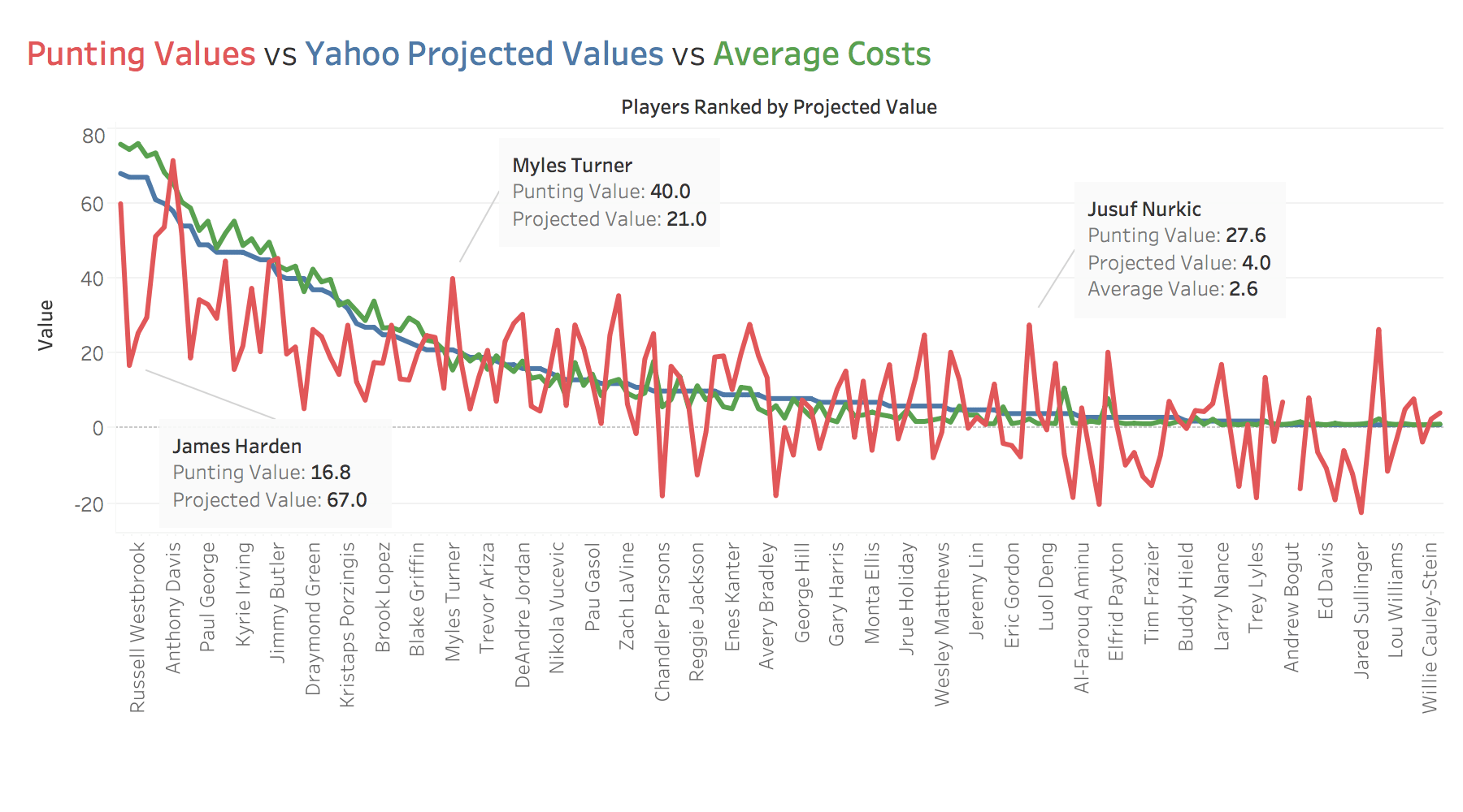
We can see in the above graph that many of the
top players lose much of their value when
discounting three pointers and assists. James
Harden for instance is one of the best
playmakers and three point scorers in the
league. His value absolutely plummets from \$67
to \$16 when we disregard his most important
stats (3pts and assists).
Players like Myles Turner and Jusuf Nurkic, however, become bargains when discounting those same stats. Jusuf Nurkic now has a value of almost \$30 and we can add him to our team for an average of only \$2.6. That type of value is absolutely insane to think about. With purchases like that we are able to receive over 10x the value for our dollar. If we can target players to create a full team of players like Jusuf Nurkic, our team can become significantly more likely to win than the average fantasy team.
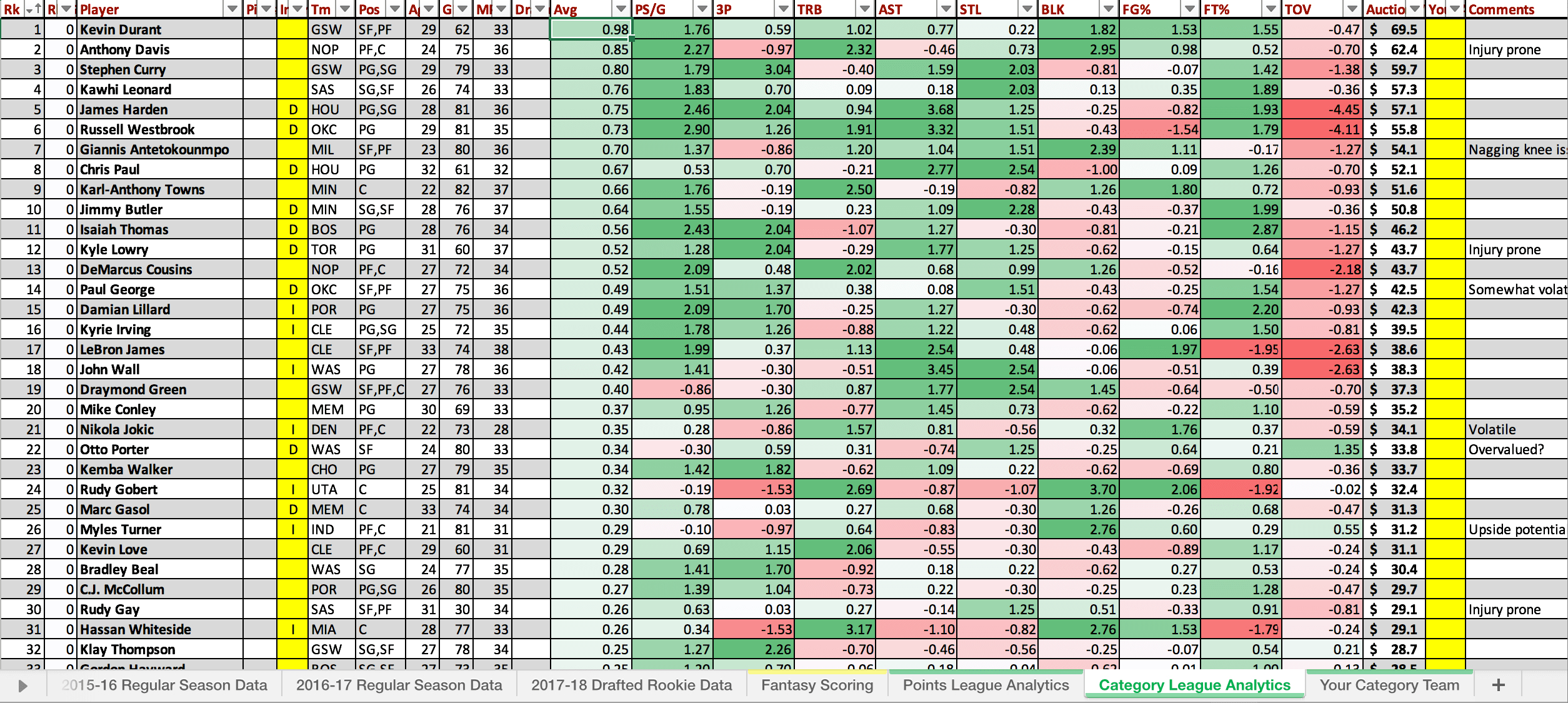
To aid in my draft I took the above data and
compiled it into an excel spreadsheet for ease
of use during draft day. Below you can see a
screenshot of the spreadsheet including a few
notes I made on players.
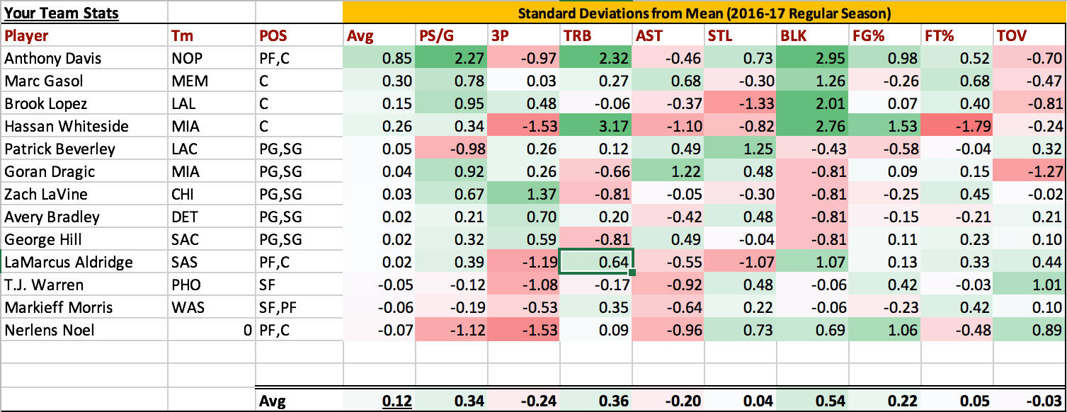
I also added a live team tracker where I can see
while drafting which categories I'm doing well
in and which need to be improved.
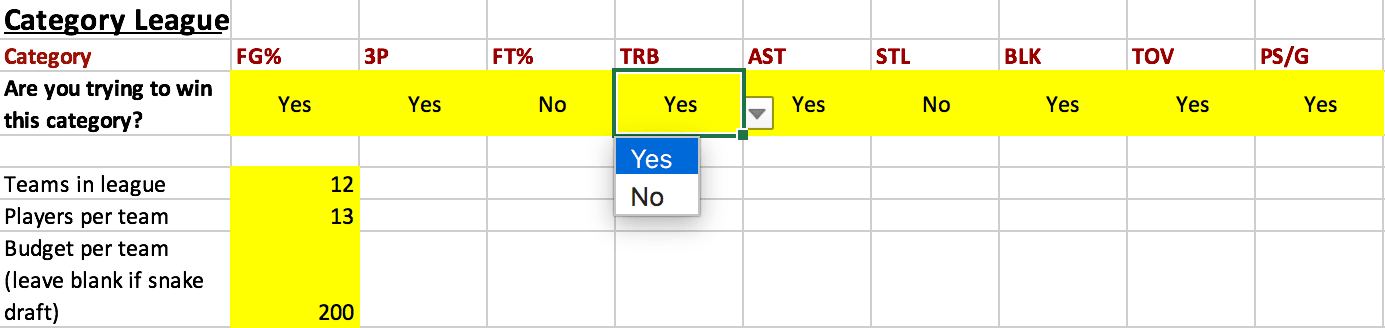
Lastly, I've added the option to select
categories to punt which will impact auction
values and average z-scores in the first table.
Ultimately, in sports nothing is a guarantee,
there are always injuries and trades that can
change player value mid season, or destroy a
team's chances, but by using z-scores we
increase our chances of winnning substantially.
Much like the Oakland As in Moneyball, you don't
need to spend the most money on players in order
to have the most competitive team.
Technical Process
First let's bring in our raw data from a CSV file downloaded from BasketballReference.com. Let's do that using the Python Pandas module.
#Importing all the needed modules for this analysis
import pandas as pd
import regex as re
from IPython.display import display_html

#This function allows for displaying dataframes side by side
def display_side_by_side(*args):
    html_str=''
    for df in args:
        html_str+=df.to_html()
    display_html(html_str.replace('table','table style="display:inline"'),raw=True)

#Here we are reading in our raw data and displaying it
df_nba = pd.read_csv("NBA_raw_data.csv", index_col=None)
df_nba.drop("Rk", axis=1, inplace=True)

#Formatting table displays
pd.options.display.max_columns = None
pd.options.display.max_rows = 10

df_nba
Ok we've imported our data but notice how there are a few things that must be cleaned up before this data is useable.
- Players that were traded mid-season currently appear as multiple rows
- Player names appear with an identifier following the name, which we don't want
Let's remove the duplicate rows for players that were traded teams. We will keep only the stats for the current team that players play for, rather than taking a weighted average between teams. This is because we only want a picture of the current situation of each player so that we can use those stats to make future decisions.
#Dropping duplicate values
df_nba.drop_duplicates(subset="Player", keep="last", inplace=True)

df_nba
#Next let's clean up the player names. We're going to the Python Regular Expressions module to do this.
pattern_to_search = r"\\[a-z | A-Z | 0-9]*"
df_nba["Player"].replace(regex=pattern_to_search, value="", inplace=True)
df_nba.set_index("Player", inplace=True)

df_nba.head()
I'm curious, let's check to see how our players did with our old "Points" scoring system that we used last year. This won't be totally accurate for this years scoring system but it should give us a general idea of where all the players stand.
Last year we didn't use category scoring. Instead stats were assigned the following number of fantasy points (FP).
Each NBA...
- Point is worth 0.5 FP
- Assist is worth 2 FP
- Rebound is worth 1.5 FP
- Block is worth 3 FP
- Steal is worth 3 FP
-
Field goal attempt (FGA) is worth -0.45
FP
-
Field goal make (FG) is worth 1 FP
-
Three point make (3P) is worth 3 FP
- Turnover is worth -2 FP
-
Free throw attempt (FTA) is worth -0.75
FP
-
Free throw make (FT) is worth 1 FP
#Creating a new column to display fantasy points generated with our old scoring system. Viewing top 10 players.
pd.set_option('display.float_format', lambda x: '%.3f' % x)
df_nba["Fantasy_pts"] = (df_nba["PS/G"] * .5) + (df_nba["AST"] * 2) + (df_nba["TRB"] * 1.5) + (df_nba["BLK"] * 3) + \
                        (df_nba["STL"] * 3) + (df_nba["3P"] * 3) + (df_nba["TOV"] * -2) + (df_nba["FGA"] * -.45) + \
                        (df_nba["FG"] * 1) + (df_nba["FTA"] * -.75) + (df_nba["FT"] * 1)

df_nba.sort_values("Fantasy_pts", ascending=False, inplace=True)


df_nba_top = df_nba.loc[df_nba.index[0:155],
                        ["PS/G","AST", "TRB", "STL", "BLK", "3P", "TOV", "FG", "FGA", "FT","FTA", "Fantasy_pts"]]

df_nba_top.head(10)
Now we can see who the top 10 players were in our league last year! That's nice but this year we're using a much more complex scoring system, so we need a new metric to evaluate players on.
Luckily the perfect metric exists to compare player value across different categories. Z-scores - that sounds complicated, I know! But let's walk through it step by step.
There are 12 participants in our league that must each select 13 NBA players for their team. That means a total of 156 NBA players must be selected out of a pool of 486 players.
We can take the average value and the standard deviation of the top 156 players in our league to see what the average value and standard deviation in each category should be. We can then compare each individual players output in each category to see how many standard deviations away from the average they are in each category. This is a z-score.
In other words if the league average number of assists is 4.5 assists. A z-score of 0.0 would mean you average exactly 4.5 assists. You are 0 standard deviations away from the mean. A z-score of 1.0 would mean you are one standard deviation above the mean, and -1.0 would mean one standard deviation below the mean assist number.
This allows us to compare categories against one another. If we wanted to see if 5 assists or 10 rebounds is more valuable, we can use z-scores to compare the two categories.
#Creating formulas to calculate z-scores for each category
def calculate_simple_zscore(series, col_name, invert_values=False):
    zscore = (series - df_nba_top[col_name].mean()) / df_nba_top[col_name].std()
    if invert_values:
        zscore = zscore * -1
    return zscore

def calculate_complex_zscore(series_makes, series_attempts, makes_col_name, attempts_col_name):
    mean_percent_made_top = df_nba_top[makes_col_name].sum() / df_nba_top[attempts_col_name].sum()
    std_percent_made_top = (df_nba_top[makes_col_name] / df_nba_top[attempts_col_name]).std()
    mean_attempts_top = df_nba_top[attempts_col_name].mean()

    series_percent_made = series_makes / series_attempts
    series_delta_from_average = series_percent_made - mean_percent_made_top
    series_zscore = series_delta_from_average / std_percent_made_top
    series_volume_multiplier = series_attempts / mean_attempts_top
    series_adjusted_zscore = series_zscore * series_volume_multiplier
    series_adjusted_zscore.rename(f"{makes_col_name}%", inplace=True)
    return series_adjusted_zscore
#Calculating z-scores
simple_stats = ["PS/G", "AST", "TRB", "STL", "BLK", "3P"]
inverted_stats = ["TOV"]
complex_stats = [("FG", "FGA"), ("FT","FTA")]

zscores_bucket = []
for col_name in simple_stats:
    result = calculate_simple_zscore(df_nba[col_name], col_name)
    zscores_bucket.append(result)

for col_name in inverted_stats:
    result = calculate_simple_zscore(df_nba[col_name], col_name, invert_values=True)
    zscores_bucket.append(result)

for pair in complex_stats:
    result = calculate_complex_zscore(df_nba[pair[0]], df_nba[pair[1]], pair[0], pair[1])
    zscores_bucket.append(result)

df_zscores = pd.concat(zscores_bucket, axis=1)

df_zscores.head(10)
Great now we can see the z-scores of each player across each category.
Next what we want to do is see overall player value for each player so we can rank them against each other. Let's simply average each of the categories to get an average z-score for each player.
#Averaging z-scores and sorting best to worst.
df_zscores["avg_zscore"] = df_zscores.mean(axis=1)

df_zscores.sort_values("avg_zscore", ascending=False)
Kevin Durant was the best player in 2016-17! We need to convert these z-scores now so that we now how much they are worth in a league using \$2400 across 12 teams drafting 156 players total.
We can calculate our auction values by assigning each z-score a percentage of the sum of the top 156 z-scores. Before doing that though, we must account for the fact that some z-score will be negative numbers. Let's first adjust up all our z-scores by the lowest negative number of the top 156 players. This sounds confusing but it maintains the percentage differece between our z-scores, which is used for calculating auction values. We can the drop these adjusted z-scores since they don't tell us anything useful.
If you didn't follow that just know that below we calculate our auction values.
#Calculating auction values based on z-scores
league_members = 12
players_per_member = 13
cash_per_member = 200


df_zscores["avg_zscore_adj"] = df_zscores["avg_zscore"] + abs(df_zscores.loc[df_zscores.index[155], ["avg_zscore"]])[0]
df_zscores["auction_value"] = (df_zscores["avg_zscore_adj"] / df_zscores.loc[df_zscores.index[0:155], ["avg_zscore_adj"]].sum()[0]) * league_members * cash_per_member
df_zscores.drop(["avg_zscore_adj"], axis=1, inplace=True)
df_zscores = df_zscores.round(2)

pd.options.display.max_rows = None
df_zscores.sort_values(["auction_value"], ascending=False).head(10)
Now let's try punting categories and see how that impacts our ending values.
Let's try punting assists and three pointers to see if big men jump in the rankings as predicted. Pay particular attention to big men such as Anthony Davis and Karl-Anthony Towns who were ranked 3rd and 10th repectively.
#Creating a function that allows us to select categories to punt
def punt_cats(df, pts=False, ast=False, trb=False, stl=False, blk=False, threes=False, tov=False, fg=False, ft=False):
    punt_category = {
        "PS/G" : pts,
        "AST" : ast,
        "TRB" : trb,
        "STL" : stl,
        "BLK" : blk,
        "3P" : threes,
        "TOV" : tov,
        "FG%" : fg,
        "FT%" : ft
    }

    df.drop(["avg_zscore", "auction_value"], axis=1, inplace=True)
    num_cats = sum(value == False for value in punt_category.values())
    df["avg_zscore"] = 0

    for cat in punt_category:
        if punt_category[cat] is False:
            df["avg_zscore"] += df[cat]

    df["avg_zscore"] = df["avg_zscore"] / num_cats
    df.sort_values("avg_zscore", ascending=False, inplace=True)

    df["avg_zscore_adj"] = df["avg_zscore"] + abs(df.loc[df.index[155], ["avg_zscore"]])[0]
    df["auction_value"] = (df["avg_zscore_adj"] / df.loc[df.index[0:155], ["avg_zscore_adj"]].sum()[0]) * league_members * cash_per_member
    df.drop(["avg_zscore_adj"], axis=1, inplace=True)
    df["auction_value"] = df["auction_value"].round(2)

punt_cats(df_zscores, ast=True, threes=True)

df_zscores.head(10)

# If you're a basketball fan you are probably wondering who Edy Tavares is at this point.
# He played 1 game last year and happened to do well in a few categories.
# We could filter out players with few games but I chose not to because then we would be screening out
# good injured players.
As expected Anthony Davis is now the best player and Karl-Anthony Towns jumped from 10th place to 3rd.
Awesome! We've reached our final values. But why not make this data set more useable for my friends. Let's make this dataset into an easy to use interface on Excel that we can use during draft day.
#Sending data into Excel
df_final = pd.concat([df_nba[["Pos", "Age", "Tm", "G", "MP"]], df_zscores], axis=1, sort=True)
df_final.to_excel("nba_stats.xlsx", sheet_name="z-scores")
Here's the end product, a table where you can
easily see who the best players are. And quickly
sort by whichever category you are looking to
improve.
I've added a team tracker where you can see
while you draft which categories you are doing
well in and which you should be focusing on
improving.
Lastly, I've added the option to select
categories to punt which will impact the auction
values and average z-scores in the first table.
To repeat the conclusion in the analysis section...
Ultimately, in sports nothing is a guarantee, there are always injuries and trades that can change player value mid season, or destroy a teams chances, but by using z-scores we increase our chances of winnning substantially. Much like the Oakland As in Moneyball, you don't need to spend the most money on players in order to have the most competitive team.