Foreword
This case is split into two parts. The first section, Analysis, discusses the high level implications of my findings. The second section, Technical Process, goes through the step by step code that I used to generate these insights.
I will be operating under the assumption that you know the basics of how chess is played. So, if you are unfamiliar with chess you may want to look at another one of my cases instead.
Analysis
I've been playing online chess for almost four years now and I've played a lot of games. On the one hand, this is great for data analysis because it gives me a large sample size with which to draw insights. But on the other hand, I am embarassed to admit just how many games I've played. This analysis will be using data from ~1,950 chess games that I've played over the last 3-4 years. Over 100,000 moves have been played across those games.
I figured that since Lichess.org offers an API to fetch personal game data it would be interesting to see what insights can be gleaned from the years I've spent playing online chess. The goal of this analysis is to discover actionable insights that I can use to improve my chess rating.
Let's take a look at how I've been doing so far. The graph below shows a breakdown of my rating over time broken out by different chess game variants. To put the rating numbers into context, someone who has just started playing chess will typically clock in at around 1000 - 1200 rating points, whereas grandmasters can be found in the 2000+ range. The current world champion, Magnus Carlsen, hovers at around 2800 rating points.
It is also important to understand the different game variations in the graph below. Classical, rapid, blitz, and bullet chess are all standard chess games but played with different time constraints. Three Check, is a variation of chess where the goal is to check your opponent three times to win.
The time constraints of classical, rapid, blitz, and bullet chess are as follows:
- Classical is any game where each side has >15 minutes to play the game.
- Rapid is between 5 and 15 minutes per side.
- Blitz is between 1 and 5 minutes per side.
- Bullet is < 1 minute per side. This sounds completely ridiculous, I know, but top chess players can somehow make it work.
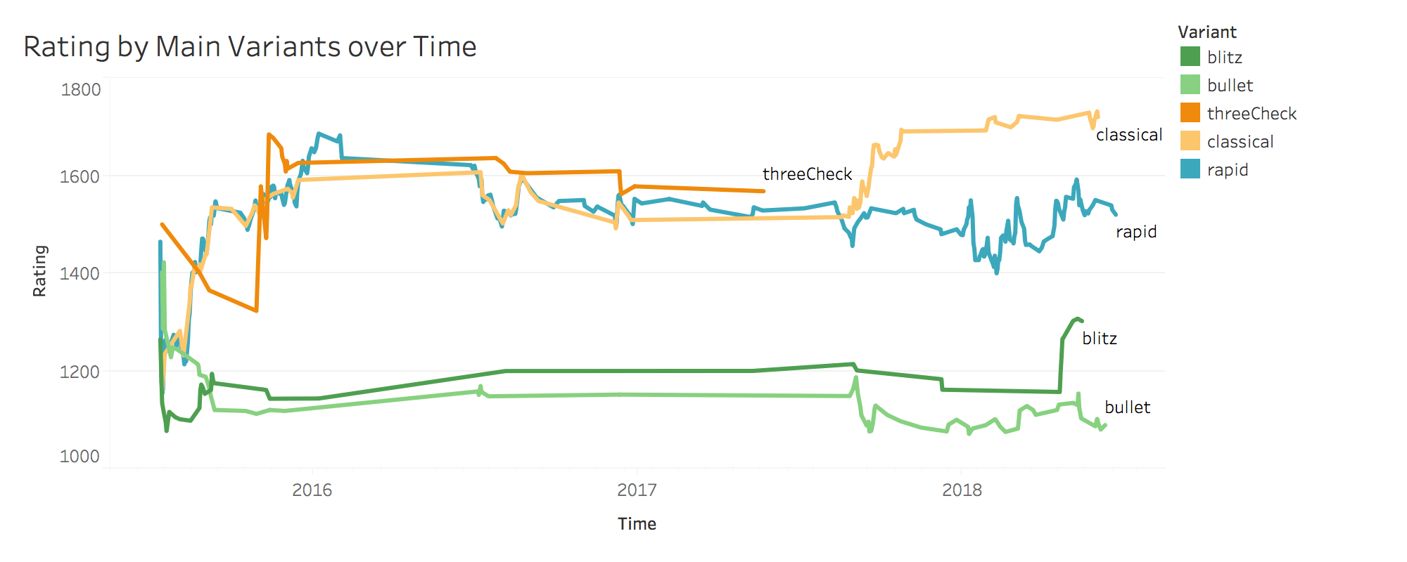
We can see that I am much weaker at faster time controls. In the 3-4 years that I've been playing, my bullet and blitz ratings have barely changed whereas my classical and rapid rating have increased to 1700 and 1500 rating points respectively.
Let's see what insights we can draw from my games to improve my ratings. To source my game data, I connected to the Lichess API and cleaned my data with Python then compiled that data into a PostGreSQL database. Detailed code can be found in the Technical Process section below.
Ok enough technical jargon, let's get my rating up.
Before even looking for ways to improve my actual chess play, I want to see if I can game the matchmaking system to artifically inflate my rating without improving my play. On Lichess, we can specify the rating range we would like our opponent to be within, so maybe I can play more often against weaker opponents to improve my rating. Let's check to see our win rates against different opponent strengths.
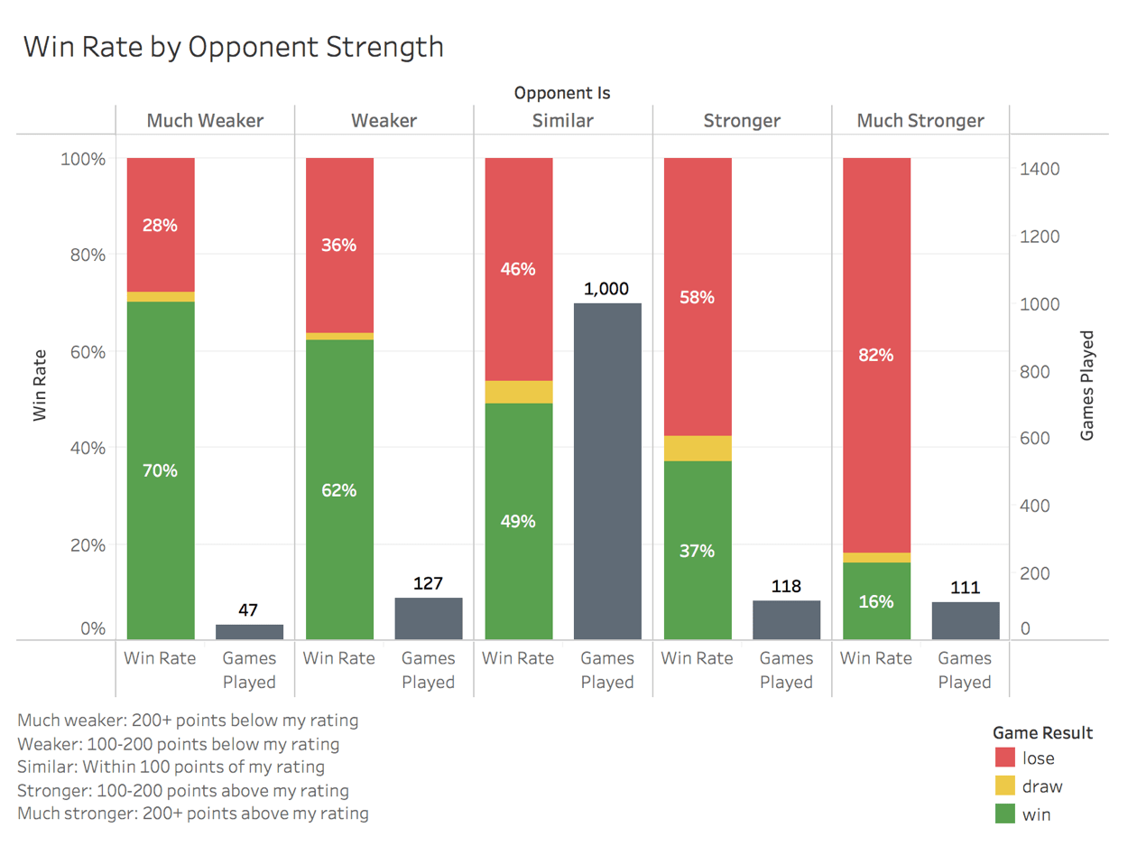
Well, right off the bat it looks like my assumption that our sample would be good enough for conclusive analysis may be false. After filtering out non-ranked games and unusual chess variations we're left with just under 1500 games. Of those 1,500 games, 1,000 of them were played against similar skill level opponents, leaving us with very small sample sizes for opponents of stronger and weaker difficulties.
Even with the small sample sizes though, we can still see a clear trend, the stronger our opponent, the lower our winning percentage. By that logic we should selectively play weaker opponents to increase our rating, right? Well, not necessarily. The rating system will award less points for a win against a weaker player while revoking significantly more points for a loss against a weaker player. Because of this, we should check our average rating gain/loss for each opponent level before assuming that a higher win rate indicates more rating points gained.
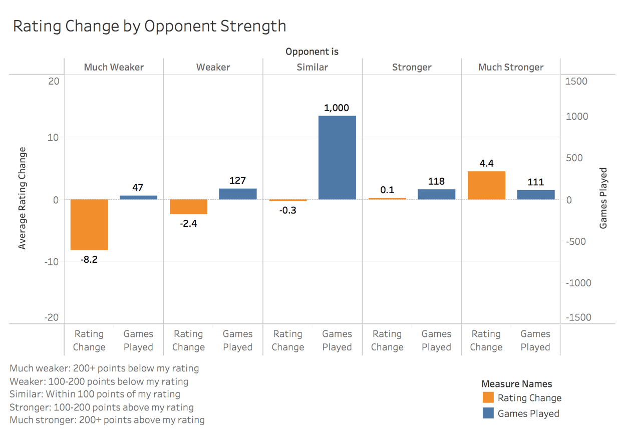
Again it's important to acknowledge that we still have problems with our sample size with this data. But we'll work with what we've got.
Counterintuitively, even though we only win 16% of games when our opponent is much stronger than us, this difficulty actually nets the largest average rating gain. Therefore we should be selectively targeting opponents with 200 or more rating points above our current level.
Conversely, we are losing almost 30% of the time when we're playing much weaker opponents. Our loss rate against very weak opponents is double our win rate against very strong opponents. Knowing this, it makes sense that we lose a ton of rating points (8 points on average) playing against very weak players. We should be avoiding playing weak opponents at all costs. Our win rate against weak opponents is not strong enough to justify the large rating loss on losing.
Ok now that we've established criteria for selecting our opponents let's take a look at our actual chess play.
At the end of every rated game on Lichess, a computer engine evaluates the strength of each move using a metric called centipawn loss (CPL). Centipawn loss is exactly what it sounds like. It is the fraction of a pawn that you are losing each move. To elaborate, if we make a move and the CPL is 100, then we have just worsened our position by the value of 1 full pawn. The goal of each move we make is to minimize centipawn loss. A CPL of 20 is considered very good.
Let's check our CPL within different game variants to see if our lower rated variants (the shorter time controls) have higher CPLs. One would expect shorter time controls to have higher average CPL since we have less time to think through our decisions.
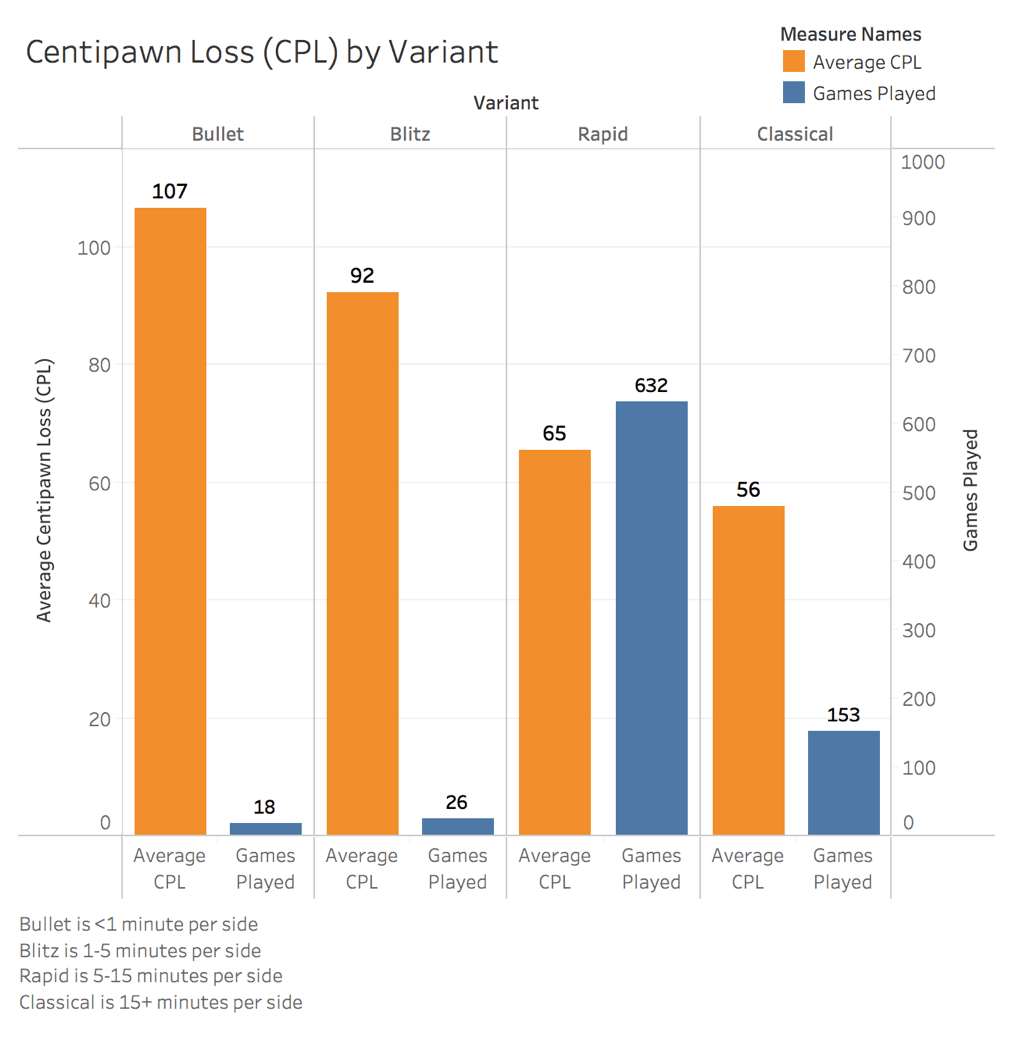
Again we've got low sample sizes for the shorter time controls, but let's be honest. We don't need data to know that 1-5 minutes per side is crazy, and will therefore yield a very high CPL. Also, note that overall sample size has decreased because CPL records are only available if requested at the time the match was played. This may inherently bias our sample, since I would only have requested CPL records for more interesting matches. We'll work with what we've got though.
As expected the longer the game, the better our decisions are. But there is nothing actionable to be taken from that knowledge, so let's see if we can segment our games by the phase of the game to see where we can improve in each variant.
Below I've broken out average CPL by the first third of the game as the opening, the second third as the middlegame, and the remaining third as the endgame.
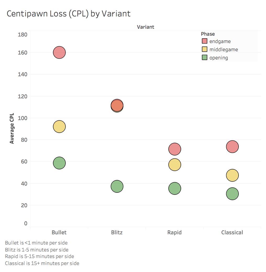
We can again see that CPL decreases as we play longer time controls, but now we can also see that we are consistently stronger during the opening and play progressively weaker moves as games progress. The endgame is our weakest phase across all time controls.
This could be a result of mental fatigue throughout the game, but it is more likely because the opening is just easier to play correctly than the sharper positions that develop later in the game. During most opening situations I will have set moves that I intend on playing because I am following a predetermined opening line. This minimizes the risk that I make any missteps during the first moves of the game. As the game progresses the position often becomes more unclear resulting in more mistakes.
It is helpful to know that I should be focusing more on training in endgame situations rather than memorizing opening sequences, as many players spend time doing. But let's see if we can look deeper into this data. I want to see which moves I am making that are causing my endgame and middlegame CPL to increase. Let's break this out further by looking at which pieces I am moving that contribute the most to my average CPL.
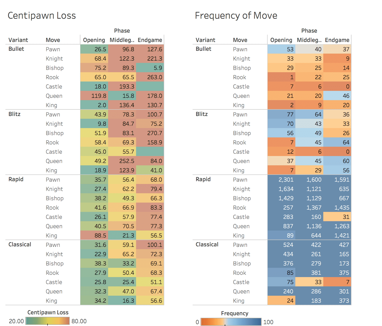
The above data visualizes why I am not good very good at bullet and blitz chess. Those quadrants of the CPL graph are a big red-orange blob of terrible moves. Granted, the sample sizes for bullet and blitz are too low to draw any meaningful conclusions.
Focusing on classical and rapid chess, however, we can see a couple of anomalies. Our endgame pawn moves in longer chess games are very weak, specifically in classical play. With an average CPL of 100, every time we move a pawn during a classical endgame, we will on average lose a pawn's worth of value. This is very actionable information - we know that we should be researching endgame pawn strategy to improve our classical rating.
We can also see that our king moves in the opening during rapid games are very weak. This makes sense, since we really shouldn't be moving our king at all during the opening. We can see this reflected on our frequency graph, where king moves in the opening are some of the least played moves in rapid and classical... But when they are played, they are usually a bad move.
We can also see on the frequency map that rarely are we castling in the middle or endgame. This makes sense and provides a nice sanity check that our data is correct. Players will almost always castle in the early game to get their king to safety. And since a player cannot castle twice, castling is usually not playable in the middle or endgame.
Outside of poor late game pawn moves in classical play, the most noticeable trend is again that my play worsens significantly from opening to middlegame and from middlegame to endgame. This is consistent across all four variants and across almost every piece type. My end game needs work.
Ultimately, I can draw a few conclusions from this analysis:
- I can artificially inflate my rating by selectively playing much stronger players than my current rating.
- My play deteriorates as the game progress. I ought to spend my time learning to end game strategies rather than focusing on opening or middlegame theory.
- In particular, my endgame pawn moves need serious improvement in longer time controls. I could take some time to study endgame pawn strategy so that I don't lose a pawn's worth of value each time I move a pawn.
In closing, I am a little disappointed at the results of this analysis. I thought I'd be able to come away with stronger conclusions by breaking out CPL by variant/piece/phase - but whether it was due to small sample size or my own chess inconsistencies, the patterns didn't seem very pronounced. I think that with a game as complicated as chess, to really glean mind blowing insights would require much more in depth analysis. For instance, if one were to integrate in a chess engine to go beyond the basic CPL metric (there are deeper chess metrics than just CPL, which weren't available to me) there would be many more possibilities to draw stronger insights.
I'll also admit that maybe I haven't played as many chess games as I first thought... I needed more data.
Technical Process
Before we can analyze anything we need to fetch our data, clean it, and store it.
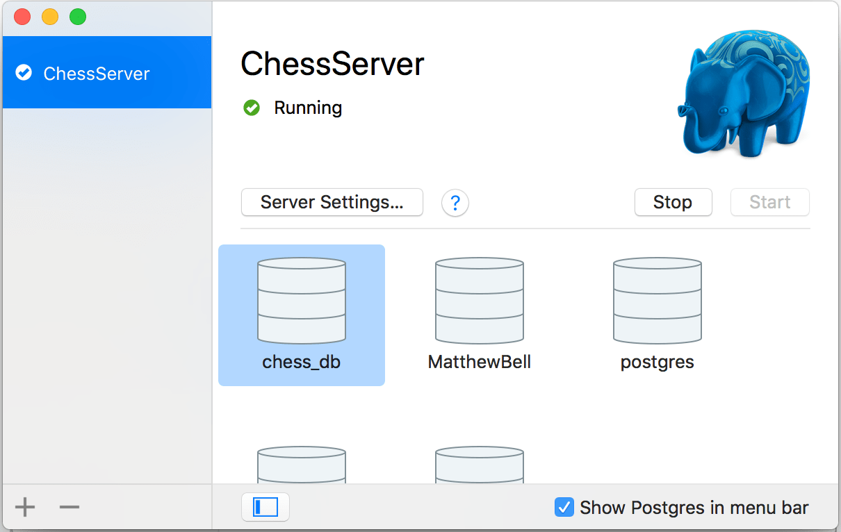
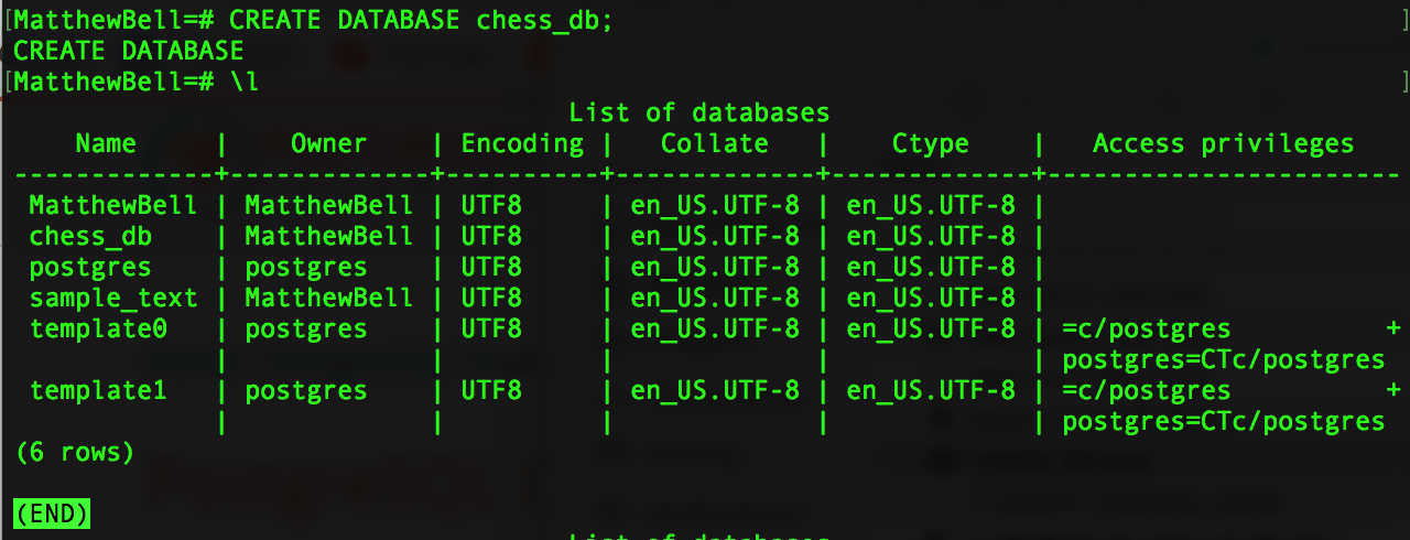
First let's create a PostGreSQL server to host our database and create a database within that server to store our data.
Next let's import all the modules we will need for this analysis. Namely we will be using Python's Pandas library for much of our data manipulation and Psycopg2 to connect to our PostGres database and to send SQL queries.
#Importing all the needed modules for this analysis
import pandas as pd
import requests, json, pickle, psycopg2, datetime
from itertools import zip_longest
from IPython.display import display_html

#This function allows for displaying dataframes side by side
def display_side_by_side(*args):
    html_str=''
    for df in args:
        html_str+=df.to_html()
    display_html(html_str.replace('table','table style="display:inline"'),raw=True)

#Formatting table displays
pd.options.display.max_columns = None
pd.options.display.max_rows = 10
Next I've written a quick Psycopg2 class to simplify connecting to our database. We will use this throughout our analysis.
#The Psycopg2 database connection class I use to connect to the database
class Database_Connection:
    def __init__(self, _dbname, _user="", _host="localhost", _password="", _port=2222):
        try:
            self.connection = psycopg2.connect(dbname=_dbname, user=_user, host=_host, password=_password, port=_port)
            self.connection.autocommit = True
            self.cursor = self.connection.cursor()
        except:
            print("Cannot connect to database\n")

    def comm(self, command, command2=None):
        self.cursor.execute(command, command2)

    def close(self):
        self.cursor.close()
        self.connection.close()
Now that we have a database to store our data let's fetch our data, clean it, and structure our database.
The script below sends a GET request to the Lichess API to fetch an NDJSON (variation of JSON) file of all of the games I've ever played, all the moves I've made, and details on the players in each of those games.
The script then converts the NDJSON file to standard JSON and the parses through the JSON file to clean the data for use in a databse. Specifically, we structure and create three data tables: 'overview', 'player_info', and 'moves'.
fetch_new_data = False
create_database = False

#Retrieves all Lichess game details from Lichess API and saves them to a JSON file
if fetch_new_data:
    url = "https://www.lichess.org/api/games/user/mbellm"
    print("Fetching game data...")
    response = requests.get(
        url,
        params={"clocks":"true", "evals":"true", "opening":"true"},
        headers={"Accept":"application/x-ndjson"})

    response = response.content.decode("utf-8")
    stripped_response = [json.loads(x) for x in response.split("\n")[:-1]]
    with open("chess_raw_data.json", "w") as f:
        json.dump(stripped_response, f, indent=2)
    print("Data Fetched.")

with open("chess_raw_data.json") as f:
    chess_games_list = json.load(f)


#Connects to database using Psycopg2 and creates tables for data insertion
if create_database:
    print("Connecting to database and creating tables...")
    chess_db = Database_Connection("chess_db")
    chess_db.comm("DROP TABLE IF EXISTS overview, moves, player_info")
    chess_db.comm("""
        CREATE TABLE overview (
        Game_ID VARCHAR (50) PRIMARY KEY,
        Game_start TIMESTAMP,
        Game_end TIMESTAMP,
        Rated BOOL NOT NULL,
        Variant VARCHAR (50),
        Speed VARCHAR (50),
        Status VARCHAR(50),
        Winner VARCHAR(50),
        Opening VARCHAR(255),
        Time_Initial INTEGER,
        Time_Increment INTEGER
        )""")
    chess_db.comm("""
        CREATE TABLE player_info (
        Index SERIAL PRIMARY KEY,
        Game_ID VARCHAR (50) NOT NULL REFERENCES overview(Game_ID),
        Username VARCHAR (50),
        Colour VARCHAR (50),
        Rating INTEGER,
        Rating_dif INTEGER,
        Inaccuracies INTEGER,
        Mistakes INTEGER,
        Blunders INTEGER,
        Average_CPL INTEGER
        )""")
    chess_db.comm("""
        CREATE TABLE moves (
        Index SERIAL PRIMARY KEY,
        Move_number INTEGER,
        Colour VARCHAR (50),
        Game_ID VARCHAR (50) NOT NULL REFERENCES overview(Game_ID),
        Move VARCHAR(10),
        Eval INTEGER,
        Forced_mate_for VARCHAR (50),
        Error_value VARCHAR (50)
        )""")
    print("Tables created.")

    #Parses through JSON file, cleans data and inserts data into tables
    count = 0
    for game in chess_games_list:
        count += 1
        print("Inserting data from game:", count)
        game_id = game["id"]
        rated = bool(game["rated"])
        variant = game["variant"]
        game_start = game["createdAt"]
        game_start = datetime.datetime.utcfromtimestamp(game_start/1000).strftime('%Y-%m-%d %H:%M:%S')
        game_end = game["lastMoveAt"]
        game_end = datetime.datetime.utcfromtimestamp(game_end/1000).strftime('%Y-%m-%d %H:%M:%S')
        speed = game["speed"]
        status = game["status"]
        try:
            opening = game["opening"]["name"]
        except:
            opening = None
        try:
            winner = game["winner"]
        except:
            winner = None
        try:
            time_initial = game["clock"]["initial"]
            time_increment = game["clock"]["increment"]
        except:
            time_initial = None
            time_increment = None

        chess_db.comm("""
        INSERT INTO overview
        (Game_ID, Game_start, Game_end, Rated, Variant, Speed, Status,
        Winner, Opening, Time_initial, Time_increment)
        VALUES (
        %s, %s, %s, %s, %s, %s, %s, %s, %s, %s, %s
        )""", (game_id, game_start, game_end, rated, variant,
            speed, status, winner, opening, time_initial, time_increment))


        for colour in game["players"]:
            try:
                user = game["players"][f"{colour}"]["user"]["name"]
            except:
                user = None

            try:
                rating = game["players"][f"{colour}"]["rating"]
                rating_dif = game["players"][f"{colour}"]["ratingDiff"]
            except:
                rating = None
                rating_dif = None

            try:
                inaccuracies = game["players"][f"{colour}"]["analysis"]["inaccuracy"]
                mistakes = game["players"][f"{colour}"]["analysis"]["mistake"]
                blunders = game["players"][f"{colour}"]["analysis"]["blunder"]
                average_cpl = game["players"][f"{colour}"]["analysis"]["acpl"]
            except:
                inaccuracies = None
                mistakes = None
                blunders = None
                average_cpl = None

            chess_db.comm("""
            INSERT INTO player_info
            (Game_ID, Username, Colour, Rating, Rating_dif, Inaccuracies,
            Mistakes, Blunders, Average_CPL)
            VALUES (
            %s, %s, %s, %s, %s, %s, %s, %s, %s
            )""", (game_id, user, colour, rating, rating_dif,
                inaccuracies, mistakes, blunders, average_cpl))

        moves = game["moves"].split(" ")
        try:
            evals = game["analysis"]
        except:
            evals = [None]

        move_number = 1
        for sequence in zip_longest(moves, evals):
            move = sequence[0]
            if move_number % 2 == 0:
                colour = "black"
            else:
                colour = "white"

            try:
                forced_mate_for = None
                evaluation = None
                evaluation = sequence[1]["eval"]
            except:
                try:
                    forced_value = sequence[1]["mate"]
                    if forced_value < 0:
                        forced_mate_for = "black"
                    else:
                        forced_mate_for = "white"
                except:
                    evaluation = None
            try:
                error_value = sequence[1]["judgment"]["name"]
            except:
                error_value = None

            chess_db.comm("""
            INSERT INTO moves
            (Move_number, Colour, Game_ID, Move, Eval,
            Forced_mate_for, Error_value)
            VALUES (
            %s, %s, %s, %s, %s, %s, %s
            )""", (move_number, colour, game_id, move,
                evaluation, forced_mate_for, error_value))

            move_number += 1
    chess_db.close()
Reconnecting to database for querying
chess_db = Database_Connection("chess_db")
Alright, we've got our database! Let's take a look at the three tables we are working with. Firstly, we have our overview table which gives us an overview of the information related to each of my 1962+ games. Yes, that's how many games I've played.
#Overview table
query = """
SELECT *
FROM overview;
"""

df = pd.read_sql(query, chess_db.connection)
df.head()
We also have our player info table which provides info on each player in each game such as their ratings and average centipawn loss for the game.
#Player_info table
query = """
SELECT *
FROM player_info
WHERE mistakes IS NOT NULL;
"""

df = pd.read_sql(query, chess_db.connection)
df.head()
Lastly we have our moves table. This one is a big one, storing over 100,000 total moves. It shows info such as the move number during each game, the move that was made, and the engine evaluation at the time that move was made.
#Moves table
query = """
SELECT *
FROM moves
WHERE error_value IS NOT NULL;
"""

df = pd.read_sql(query, chess_db.connection)
df.head()
Let's start by sending a query to check our ratings over time for each game variant where we've played at least 10 games. We need to clean up our variant and speed columns to view this since we want to break out the 'standard' variant by time control but we want to keep variants such as 'three check' labeled by their variant name.
query = """
SELECT game_start, rating,
    CASE
        WHEN variant != 'standard' THEN variant
        WHEN variant = 'standard' THEN speed
    END AS g_mode
FROM overview
JOIN player_info
ON overview.game_id = player_info.game_id
WHERE rated IS TRUE AND username = 'mbellm'
    AND CASE
        WHEN variant != 'standard' THEN variant
        WHEN variant = 'standard' THEN speed
    END IN (
        SELECT game_mode FROM (
            SELECT count(*) AS frequency,
                CASE
                    WHEN variant != 'standard' THEN variant
                    WHEN variant = 'standard' THEN speed
                END AS game_mode
                FROM player_info
                JOIN overview
                ON player_info.game_id = overview.game_id
                    AND player_info.username = 'mbellm'
                    AND rated IS TRUE
            GROUP BY 2
            HAVING count(*) > 10) inner_q)
"""

df = pd.read_sql(query, chess_db.connection)
df
Great, now let's check our win rate against different opponent strengths. We'll buckets our games into five difficulty levels to see our win, losses, and draws at each level. This will make it easy for us to graph our our results as a percentage of the total games played at each difficulty for our analysis section
#Lastly we have our moves table which has all the moves that were made in every game I've every played.
query = """
SELECT count(*) AS frequency,
    CASE
        WHEN rating_dif  < -200 THEN 'much stronger'
        WHEN rating_dif BETWEEN -199 AND -101  THEN 'stronger'
        WHEN rating_dif BETWEEN -100 AND 100 THEN 'similar'
        WHEN rating_dif BETWEEN 101 AND 199 THEN 'weaker'
        WHEN rating_dif > 200 THEN 'much weaker'
    END AS opponent_is,
    CASE
        WHEN colour = winner THEN 'win'
        WHEN colour != winner THEN 'lose'
        WHEN winner IS NULL THEN 'draw'
    END AS game_result
FROM (
    SELECT a.game_id, a.username, b.username AS opp_name, a.colour, a.rating AS my_rating,
        b.rating AS opp_rating, a.rating-b.rating AS rating_dif
    FROM player_info AS a
    JOIN player_info AS b
    ON a.game_id = b.game_id
        AND a.username = 'mbellm'
        AND b.username != 'mbellm') p_info
JOIN overview
ON overview.game_id = p_info.game_id
    AND overview.rated IS TRUE
    AND overview.variant = 'standard'
GROUP BY 2, 3
HAVING
    CASE
        WHEN rating_dif  < -200 THEN 'much stronger'
        WHEN rating_dif BETWEEN -199 AND -101  THEN 'stronger'
        WHEN rating_dif BETWEEN -100 AND 100 THEN 'similar'
        WHEN rating_dif BETWEEN 101 AND 199 THEN 'weaker'
        WHEN rating_dif > 200 THEN 'much weaker'
    END IS NOT NULL
ORDER BY 2, 3
"""

pd.options.display.max_rows = 15
df = pd.read_sql(query, chess_db.connection)
df
Next let's query the actual rating gained or lost by those same buckets, since as discussed in the analysis section, win rate does not tell the full story.
query = """
SELECT count(*) AS frequency, round(avg(rating_gain), 2) AS avg_rating_gain,
    CASE
        WHEN rating_dif  < -200 THEN 'much stronger'
        WHEN rating_dif BETWEEN -199 AND -101  THEN 'stronger'
        WHEN rating_dif BETWEEN -100 AND 100 THEN 'similar'
        WHEN rating_dif BETWEEN 101 AND 199 THEN 'weaker'
        WHEN rating_dif > 200 THEN 'much weaker'
    END AS opp_rating
FROM (
    SELECT a.game_id, a.username, b.username AS opp_name, a.colour, a.rating AS my_rating,
        b.rating AS opp_rating, a.rating-b.rating AS rating_dif, a.rating_dif AS rating_gain
    FROM player_info AS a
    JOIN player_info AS b
    ON a.game_id = b.game_id
        AND a.username = 'mbellm'
        AND b.username != 'mbellm') p_info
JOIN overview
ON overview.game_id = p_info.game_id
    AND overview.rated IS TRUE
    AND overview.variant = 'standard'
GROUP BY 3
HAVING
    CASE
        WHEN rating_dif  < -200 THEN 'much stronger'
        WHEN rating_dif BETWEEN -199 AND -101  THEN 'stronger'
        WHEN rating_dif BETWEEN -100 AND 100 THEN 'similar'
        WHEN rating_dif BETWEEN 101 AND 199 THEN 'weaker'
        WHEN rating_dif > 200 THEN 'much weaker'
    END IS NOT NULL
ORDER BY 3;
"""

df = pd.read_sql(query, chess_db.connection)
df
I thought it would be interesting to also graph out the win rate depending on which move I castled as well. I thought that perhaps games where I delayed castling would have lower win rates as my king would be less safe.
#When should I be castling
query = """
SELECT move_number,
    CASE
        WHEN colour = winner THEN 'win'
        WHEN winner IS NULL THEN 'draw'
        WHEN colour != winner THEN 'lose'
    END AS game_res, count(*) AS frequency
FROM (
    SELECT moves.game_id, move_number, moves.colour
    FROM moves
    JOIN player_info
    ON moves.game_id = player_info.game_id
        AND player_info.username = 'mbellm'
        AND moves.colour = player_info.colour
        AND (moves.move = 'O-O' OR moves.move='O-O-O')) inner_q
JOIN overview
ON inner_q.game_id = overview.game_id
    AND overview.variant = 'standard'
GROUP BY 1,2
ORDER BY 1,2
"""
pd.options.display.max_rows = 10
df = pd.read_sql(query, chess_db.connection)
df_grouped = df.groupby('move_number').agg('sum')
df.to_csv('castling_data.csv')
df_grouped.to_csv('castling_data_grouped.csv')
df
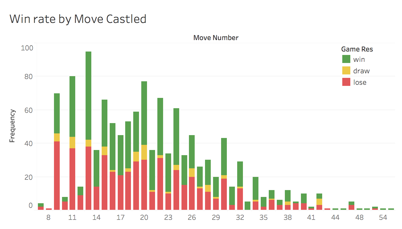
As we can see from the graph above however, there was not much of a trend to this data so I omitted it from the analysis. We can see that the openings I play usually result on castling on move 9, 11, or 13. But there isn't much to be done with that information.
Next let's check to see how we do during differently time controls. I expect faster time controls to have higher average centipawn loss.
#Average CPL by speed
query ="""
SELECT count(*) AS frequency, round(avg(average_cpl),2) AS avg_cpl, speed
FROM player_info
JOIN overview
ON player_info.game_id = overview.game_id
WHERE username = 'mbellm' AND inaccuracies IS NOT NULL
GROUP BY variant, speed
HAVING variant = 'standard' AND speed NOT IN ('correspondence', 'ultraBullet')
ORDER BY avg_cpl
"""

df = pd.read_sql(query, chess_db.connection)
df
As expected bullet is our worst variant and classical is our best.
But what about if we break those time controls out by the phase of the game, do I need to work on a certain parts of my game more than others?
To split avg CPL by game phase we need to first calculate average centipawn loss per move by taking the difference between engine evaluations on each move. In order to do that we need to clean up a couple of engine evaluation errors for when white/black is in a checkmate position, let's update our table first then calculate CPL per move.
#Updating table to be able to calculate avg cpl
query = """
UPDATE moves
SET eval =
        CASE
            WHEN forced_mate_for = 'white' THEN 1000
            WHEN forced_mate_for = 'black' THEN -1000
            WHEN eval IS NULL THEN NULL
            WHEN eval > 1000 THEN 1000
            WHEN eval < -1000 THEN 1000
            ELSE eval
        END
"""

chess_db.comm(query)
#Calculating cpl per move
query = """
SELECT player_info.game_id, move_number, move, player_info.colour, cpl AS avg_centi
FROM (
    SELECT *,
        CASE
            WHEN colour = 'white' THEN (eval - lag(eval) OVER
                (PARTITION BY game_id ORDER BY game_id, move_number)) *-1
            WHEN colour = 'black' THEN (eval - lag(eval) OVER (PARTITION BY game_id ORDER BY game_id, move_number))
        END AS cpl
FROM moves ) inner_q
JOIN player_info
ON inner_q.game_id = player_info.game_id AND inner_q.colour = player_info.colour
WHERE player_info.game_id != '02EW8kec'
ORDER BY player_info.game_id, move_number
"""

df = pd.read_sql(query, chess_db.connection)
df
Now that our table is updated with CPL per move, I've created a function that will split each game into thirds. The function takes the max number of moves in each game and sets break points for the opening, middlegame, and endgame. Then it adds a phase column for each move.
def define_move_phase(x):
    bins = (0, round(x['move_number'].max() * 1/3), round(x['move_number'].max() * 2/3), x['move_number'].max())
    phases = ["opening", "middlegame", "endgame"]
    try:
        x.loc[:, 'phase'] = pd.cut(x['move_number'], bins, labels=phases)
    except ValueError:
        x.loc[:, 'phase'] = None
    return x

df = df.groupby('game_id').apply(define_move_phase)
df
Now we need to join our player_info, overiew, and moves tables together to view avg cpl by piece moved by variant by phase. Let's first join overview and player_info together then add those to our moves table.
#Filter data to where it's only my games
query = """
SELECT player_info.game_id, username, colour, variant, speed
FROM player_info
JOIN overview
ON player_info.game_id = overview.game_id
"""

df2 = pd.read_sql(query, chess_db.connection)
print(df2.shape)
df2.head()
Now let's join those tables onto our moves table and filter out moves made by our opponents now that we can who made each move. My username is 'mbellm' which is being filtered.
df = pd.merge(df,df2,on=['game_id', 'colour'])
df = df[(df['username'] == 'mbellm')]
df
Let's clean up our variant column again, this time using pandas. Let's replace the 'standard' variant type with the associated time controls for each move.
try:
    m = df['variant'] == 'standard'
    df.loc[m, 'variant'] = df.loc[m, 'speed']
    df.drop('speed', axis=1, inplace=True)
except KeyError:
    pass
df = df[(df['variant'] == 'rapid') | (df['variant'] == 'classical') | (df['variant'] == 'bullet') |
        (df['variant'] == 'blitz')]

df
Great! Now let's check our avg CPL by game phase by variant
pd.options.display.max_rows = 20
df_loss_by_variant = df.groupby(['phase', 'variant']).agg('mean')['avg_centi']
df_loss_by_variant.loc[['opening', 'middlegame', 'endgame']]
df_loss_by_variant.to_excel("cpl_by_variant_by_phase.xlsx")
df_loss_by_variant
Now let's drill down deeper and reformat our move column so we can view the piece that was moved on each row.
pd.options.mode.chained_assignment = None
pd.options.display.max_rows = 10
def which_piece_moved(x):
    move_dict = {
        'Q' : 'Queen',
        'B' : 'Bishop',
        'N' : 'Knight',
        'K' : 'King',
        'R' : 'Rook',
        'O' : 'Castle'
    }

    if x[:1] in move_dict.keys():
        return move_dict[x[:1]]
    else:
        return 'Pawn'

df.loc[:, 'move'] = df.loc[:, 'move'].apply(which_piece_moved)
df
Now let's check our avg CPL by variant by game phase by piece moved! That's a lot of information, it should be easier to understand if we visualize that data in our analysis section.
pd.options.display.max_rows = 100
df = df.groupby(['phase', 'variant', 'move']).agg(['mean', 'count'])['avg_centi']
df.to_excel("final.xlsx")
df
Lastly, let's close out our connection to the database
chess_db.close()
To repeat the conclusion in our analysis section...
Ultimately, I can draw a few conclusions from this analysis:
- I can artificially inflate my rating by selectively playing much stronger players than my current rating.
- My play deteriotes as the game progress. I ought to spend my time learning to end game strategies rather than focusing on the opening or middlegame theory.
- In particular, my endgame pawn moves need serious improvement in longer time controls. I could take some time to study endgame pawn strategy so that I don't lose a pawn's worth of value each time I move a pawn.
In closing, I am a little disappointed at the results of this analysis. I thought I'd be able to come away with stronger conclusions by breaking out CPL by variant/piece/phase - but whether it was due to small sample size or my own chess inconsistencies, the patterns didn't seem very pronounced. I think that with a game as complicated as chess, to really glean mind blowing insights would require much more in depth analysis. For instance, if one were to integrate in a chess engine to go beyond the basic CPL metric (there are deeper chess metrics than just CPL, which weren't available to me) there would be many more possibilities to draw stronger insights.
I'll also admit that maybe I haven't played as many chess games as I first thought... I needed more data.